Deep reinforcement learning: where to start
Deep reinforcement learning: where to start
This post previously appeared on medium.
Last year, DeepMind’s AlphaGo beat Go world champion Lee Sedol 4–1. More than 200 million people watched as reinforcement learning (RL) took to the world stage. A few years earlier, DeepMind had made waves with a bot that could play Atari games. The company was soon acquired by Google.
Many researchers believe that RL is our best shot at creating artificial general intelligence. It is an exciting field, with many unsolved challenges and huge potential.
Although it can appear challenging at first, getting started in RL is actually not so difficult. In this article, we will create a simple bot with Keras that can play a game of Catch.
The game
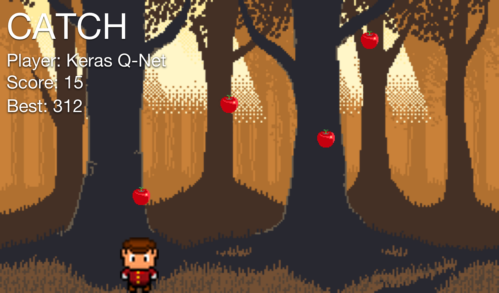 A prettier version of the game we will actually train on
Catch is a very simple arcade game, which you might have played as a child. Fruits fall from the top of the screen, and the player has to catch them with a basket. For every fruit caught, the player scores a point. For every fruit lost, the player loses a point.
The goal here is to let the computer play Catch by itself. But we will not use the pretty game above. Instead, we will use a simplified version to make the task easier:
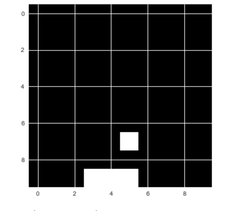 Our simplified catch game
While playing Catch, the player decides between three possible actions. They can move the basket to the left, to the right, or stay put.
The basis for this decision is the current state of the game. In other words: the positions of the falling fruit and of the basket.
Our goal is to create a model, which, given the content of the game screen, chooses the action which leads to the highest score possible.
This task can be seen as a simple classification problem. We could ask expert human players to play the game many times and record their actions. Then, we could train a model to choose the ‘correct’ action that mirrors the expert players.
But this is not how humans learn. Humans can learn a game like Catch by themselves, without guidance. This is very useful. Imagine if you had to hire a bunch of experts to perform a task thousands of times every time you wanted to learn something as simple as Catch! It would be expensive and slow.
In reinforcement learning, the model trains from experience, rather than labeled data.
Deep reinforcement learning
Reinforcement learning is inspired by behavioral psychology.
Instead of providing the model with ‘correct’ actions, we provide it with rewards and punishments. The model receives information about the current state of the environment (e.g. the computer game screen). It then outputs an action, like a joystick movement. The environment reacts to this action and provides the next state, alongside with any rewards.
The model then learns to find actions that lead to maximum rewards.
There are many ways this can work in practice. Here, we are going to look at Q-Learning. Q-Learning made a splash when it was used to train a computer to play Atari games. Today, it is still a relevant concept. Most modern RL algorithms are some adaptation of Q-Learning.
Q-learning intuition
A good way to understand Q-learning is to compare playing Catch with playing chess.
In both games you are given a state, S. With chess, this is the positions of the figures on the board. In Catch, this is the location of the fruit and the basket.
The player then has to take an action, A. In chess, this is moving a figure. In Catch, this is to move the basket left or right, or remain in the current position.
As a result, there will be some reward R, and a new state S’.
The problem with both Catch and chess is that the rewards do not appear immediately after the action.
In Catch, you only earn rewards when the fruits hit the basket or fall on the floor, and in chess you only earn a reward when you win or lose the game. This means that rewards are sparsely distributed. Most of the time, R will be zero.
When there is a reward, it is not always a result of the action taken immediately before. Some action taken long before might have caused the victory. Figuring out which action is responsible for the reward is often referred to as the credit assignment problem.
Because rewards are delayed, good chess players do not choose their plays only by the immediate reward. Instead, they choose by the expected future reward.
For example, they do not only think about whether they can eliminate an opponent’s figure in the next move. They also consider how taking a certain action now will help them in the long run.
In Q-learning, we choose our action based on the highest expected future reward. We use a “Q-function” to calculate this. This is a math function that takes two arguments: the current state of the game, and a given action.
We can write this as: Q(state, action)
While in state S, we estimate the future reward for each possible action A. We assume that after we have taken action A and moved to the next state S’, everything works out perfectly.
The expected future reward Q(S,A) for a given a state S and action A is calculated as the immediate reward R, plus the expected future reward thereafter Q(S',A'). We assume the next action A' is optimal.
Because there is uncertainty about the future, we discount Q(S’,A’) by the factor gamma γ.
Q(S,A) = R + γ * max Q(S’,A’)
Good chess players are very good at estimating future rewards in their head. In other words, their Q-function Q(S,A) is very precise.
Most chess practice revolves around developing a better Q-function. Players peruse many old games to learn how specific moves played out in the past, and how likely a given action is to lead to victory.
But how can a machine estimate a good Q-function? This is where neural networks come into play.
Regression after all
When playing a game, we generate lots of “experiences”. These experiences consist of:
- the initial state,
S - the action taken,
A - the reward earned,
R - and the state that followed,
S’
These experiences are our training data. We can frame the problem of estimating Q(S,A) as a regression problem. To solve this, we can use a neural network.
Given an input vector consisting of S and A, the neural net is supposed to predict the value of Q(S,A) equal to the target: R + γ * max Q(S’,A’).
If we are good at predicting Q(S,A) for different states S and actions A, we have a good approximation of the Q-function. Note that we estimate Q(S’,A’) through the same neural net as Q(S,A).
The training process
Given a batch of experiences < S, A, R, S’ >, the training process then looks as follows:
- For each possible action
A’(left, right, stay), predict the expected future rewardQ(S’,A’)using the neural net - Choose the highest value of the three predictions as
max Q(S’,A’) - Calculate
r + γ * max Q(S’,A’). This is the target value for the neural net - Train the neural net using a loss function. This is a function that calculates how near or far the predicted value is from the target value. Here, we will use
0.5 * (predicted_Q(S,A) — target)²as the loss function.
During gameplay, all the experiences are stored in a replay memory. This acts like a simple buffer in which we store < S, A, R, S’ > pairs. The experience replay class also handles preparing the data for training. Check out the code below:
class ExperienceReplay(object):
    """
    During gameplay all the experiences < s, a, r, s’ > are stored in a replay memory.
    In training, batches of randomly drawn experiences are used to generate the input and target for training.
    """
    def __init__(self, max_memory=100, discount=.9):
        """
        Setup
        max_memory: the maximum number of experiences we want to store
        memory: a list of experiences
        discount: the discount factor for future experience

        In the memory the information whether the game ended at the state is stored seperately in a nested array
        [...
        [experience, game_over]
        [experience, game_over]
        ...]
        """
        self.max_memory = max_memory
        self.memory = list()
        self.discount = discount

    def remember(self, states, game_over):
        #Save a state to memory
        self.memory.append([states, game_over])
        #We don't want to store infinite memories, so if we have too many, we just delete the oldest one
        if len(self.memory) > self.max_memory:
            del self.memory[0]

    def get_batch(self, model, batch_size=10):

        #How many experiences do we have?
        len_memory = len(self.memory)

        #Calculate the number of actions that can possibly be taken in the game
        num_actions = model.output_shape[-1]

        #Dimensions of the game field
        env_dim = self.memory[0][0][0].shape[1]

        #We want to return an input and target vector with inputs from an observed state...
        inputs = np.zeros((min(len_memory, batch_size), env_dim))

        #...and the target r + gamma * max Q(s’,a’)
        #Note that our target is a matrix, with possible fields not only for the action taken but also
        #for the other possible actions. The actions not take the same value as the prediction to not affect them
        targets = np.zeros((inputs.shape[0], num_actions))

        #We draw states to learn from randomly
        for i, idx in enumerate(np.random.randint(0, len_memory,
                                                  size=inputs.shape[0])):
            """
            Here we load one transition <s, a, r, s’> from memory
            state_t: initial state s
            action_t: action taken a
            reward_t: reward earned r
            state_tp1: the state that followed s’
            """
            state_t, action_t, reward_t, state_tp1 = self.memory[idx][0]

            #We also need to know whether the game ended at this state
            game_over = self.memory[idx][1]

            #add the state s to the input
            inputs[i:i+1] = state_t

            # First we fill the target values with the predictions of the model.
            # They will not be affected by training (since the training loss for them is 0)
            targets[i] = model.predict(state_t)[0]

            """
            If the game ended, the expected reward Q(s,a) should be the final reward r.
            Otherwise the target value is r + gamma * max Q(s’,a’)
            """
            #  Here Q_sa is max_a'Q(s', a')
            Q_sa = np.max(model.predict(state_tp1)[0])

            #if the game ended, the reward is the final reward
            if game_over:  # if game_over is True
                targets[i, action_t] = reward_t
            else:
                # r + gamma * max Q(s’,a’)
                targets[i, action_t] = reward_t + self.discount * Q_sa
        return inputs, targets
Defining the model
Now it is time to define the model that will learn a Q-function for Catch.
We are using Keras as a front end to Tensorflow. Our baseline model is a simple three-layer dense network.
Already, this model performs quite well on this simple version of Catch. Head over to GitHub for the full implementation. You can experiment with more complex models to see if you can get better performance.
num_actions = 3  # [move_left, stay, move_right]
hidden_size = 100 # Size of the hidden layers
grid_size = 10 # Size of the playing field

def baseline_model(grid_size,num_actions,hidden_size):
    #seting up the model with keras
    model = Sequential()
    model.add(Dense(hidden_size, input_shape=(grid_size**2,), activation='relu'))
    model.add(Dense(hidden_size, activation='relu'))
    model.add(Dense(num_actions))
    model.compile(sgd(lr=.1), "mse")
    return model
Exploration
A final ingredient to Q-Learning is exploration.
Everyday life shows that sometimes you have to do something weird and/or random to find out whether there is something better than your daily trot.
The same goes for Q-Learning. Always choosing the best option means you might miss out on some unexplored paths. To avoid this, the learner will sometimes choose a random option, and not necessarily the best.
Now we can define the training method:
def train(model,epochs):
# Train
#Reseting the win counter
win_cnt = 0
# We want to keep track of the progress of the AI over time, so we save its win count history
win_hist = []
#Epochs is the number of games we play
for e in range(epochs):
loss = 0.
#Resetting the game
env.reset()
game_over = False
# get initial input
input_t = env.observe()
while not game_over:
#The learner is acting on the last observed game screen
#input_t is a vector containing representing the game screen
input_tm1 = input_t
#Take a random action with probability epsilon
if np.random.rand() <= epsilon:
#Eat something random from the menu
action = np.random.randint(0, num_actions, size=1)
else:
#Choose yourself
#q contains the expected rewards for the actions
q = model.predict(input_tm1)
#We pick the action with the highest expected reward
action = np.argmax(q[0])
# apply action, get rewards and new state
input_t, reward, game_over = env.act(action)
#If we managed to catch the fruit we add 1 to our win counter
if reward == 1:
win_cnt += 1
#Uncomment this to render the game here
#display_screen(action,3000,inputs[0])
"""
The experiences < s, a, r, s’ > we make during gameplay are our training data.
Here we first save the last experience, and then load a batch of experiences to train our model
"""
# store experience
exp_replay.remember([input_tm1, action, reward, input_t], game_over)
# Load batch of experiences
inputs, targets = exp_replay.get_batch(model, batch_size=batch_size)
# train model on experiences
batch_loss = model.train_on_batch(inputs, targets)
#sum up loss over all batches in an epoch
loss += batch_loss
win_hist.append(win_cnt)
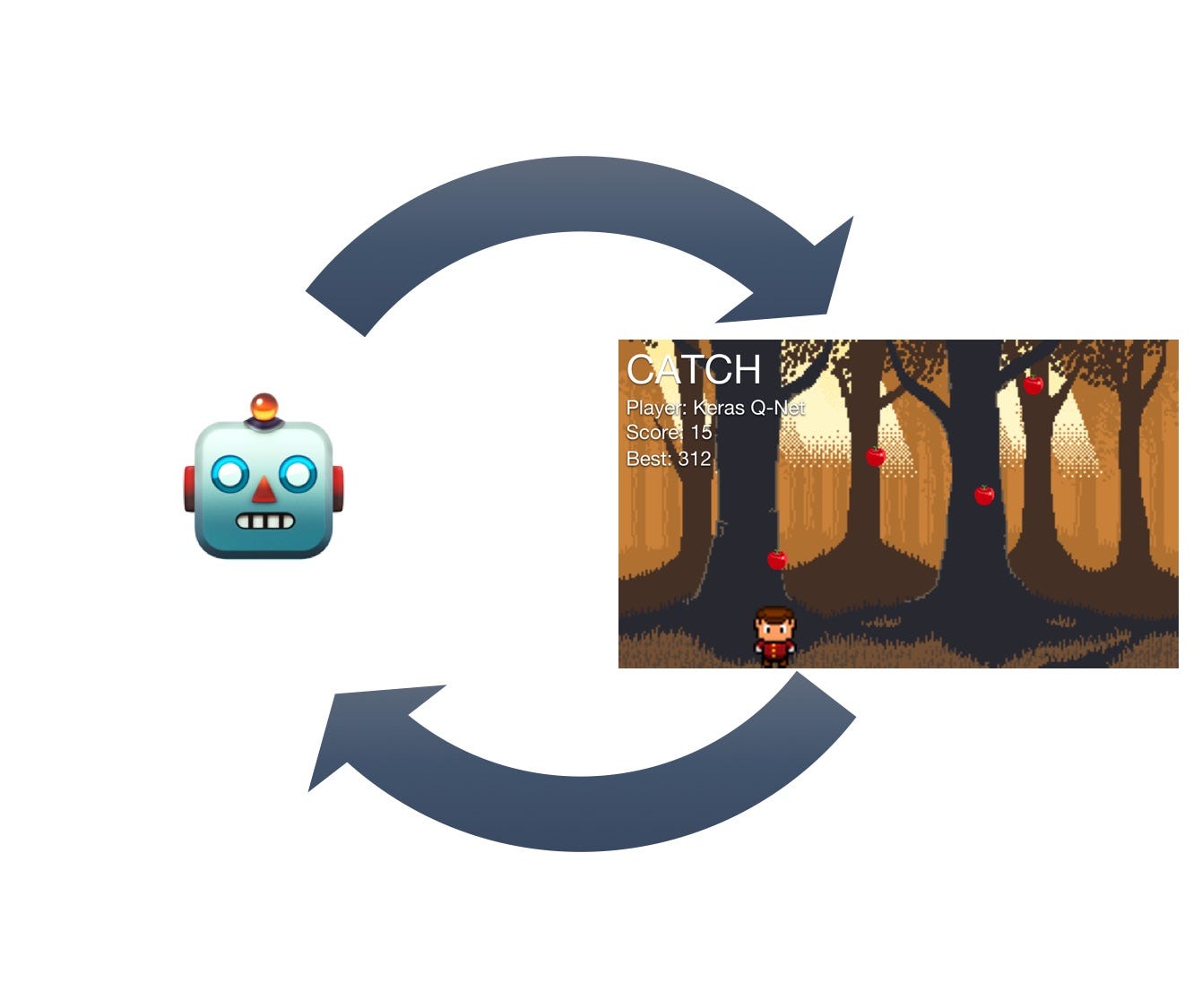
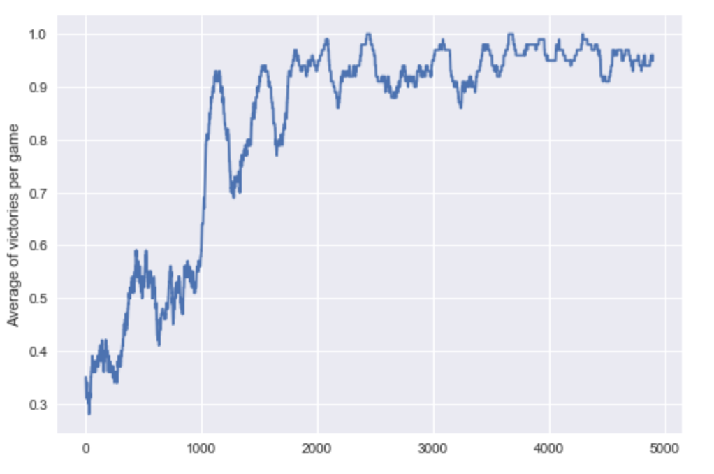
return win_histI let the game train for 5,000 epochs, and it does quite well now!
 Our Catch player in action
As you can see in the animation, the computer catches the apples falling from the sky.
To visualize how the model learned, I plotted the moving average of victories over the epochs:
Where to go from here
You now have gained a first overview and an intuition of RL. I recommend taking a look at the full code for this tutorial. You can experiment with it.
You might also want to check out Arthur Juliani’s series. If you’d like a more formal introduction, have a look at Stanford’s CS 234, Berkeley’s CS 294 or David Silver’s lectures from UCL.
A great way to practice your RL skills is OpenAI’s Gym, which offers a set of training environments with a standardized API.
Acknowledgements
This article builds upon Eder Santana’s simple RL example, from 2016. I refactored his code and added explanations in a notebook I wrote earlier in 2017. For readability on Medium, I only show the most relevant code here. Head over to the notebook or Eder’s original post for more.
About Jannes Klaas
This text is part of the Machine Learning in Financial Context course material, which helps economics and business students understand machine learning.
I spent a decade building software and am now on the journey bring ML to the financial world. I study at the Rotterdam School of Management and have done research with the Institute for Housing and Urban development studies.
You can follow me on Twitter. If you have any questions or suggestions please leave a comment or ping me on Medium.