Why business needs causal inference

Why business needs causal inference

This post is an ad. Not for a product, but for a method. Causal inference has made large strides in the last few years. It has arrived at a point, where business analysts can reason about and determine causal effects by following a few simple rules. Much of the causal inference literature is focused on medicine and public health. Economics has a long tradition of causal inference methods, but many of the traditional econometric methods are not simple enough to be used widely. Modern methods are much simpler to use. This text provides brief overview of causal inference and how it is relevant to business.

When do you need causal inference?

Sometimes correlation is just fine

Imagine you are planing your beach holiday and want to stay in a nice hotel at a time when the beach is not very busy. You have access to a dataset of bookings and hotel prices and find the following (the numbers in this example are continuous only for nice plotting and the example would work just as well with discrete variables):

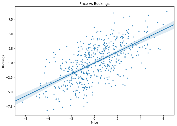
Neat! It seems like there are fewer people at the beach when hotels are cheap. This makes perfect sense since it is probably off season. You can now use this information to optimize your holidays. It is not your hotel, you do not make the prices.

But if you plan to act, you should care about causality

Now, picture that you own the hotel and want to optimize pricing. Should you raise prices to attract more customers? Obviously not. When we plan to intervene, we need to take causality into account. In this case we want to find the so called interventional distribution. Interventions matter so much that they are now key to the definition of causality in the field of causal inference. X causes Y if we can change Y by changing X. To make clear that we are manipulating X, we write P(Y|do(X)) to note the interventional distribution, which the hotel owner cares about, and P(Y|X) to note the associative distribution, which the tourist cares about.

Business analysts often work to aid management decision making. Business decisions are usually about intervention: How much should we charge? Which ad should we display? What should our product do? How do we organize our supply chain? For all decisions in which your intervention will have an effect on the outcome, you will need to make causal statements.

Causality needs good communication

You, the hotel owner, got the message and are eager to make some proper causal statements. But when does correlation become causation? I will let you in on a dirty secret here: Correlation does become causation when we assume it does. You read that right. There is no higher god of statistics showing us exactly when X causes Y and when they are merely correlated. We could look at the chart above and say: “This correlation exists because higher prices actually do attract more visitors!”.

However, it would be hard to justify this assumption. Prices and bookings are confounded by season. We therefore need to adjust our our estimate of the price effect.

Finding the right variable to adjust for is easier said than done. Should we adjust only for season, or maybe also for the ratings of the hotel, or the country it is located in? Even seasoned researchers are often not sure how all variables they are working with are fitting together. Often, researchers end up simply adjusting for every variable they can find. Blindly adjusting for all possible variables can actually induce bias and lead to faulty estimates. We will soon discuss ways in which this happens. A tool to precisely reason about causal effects and find the necessary adjustments was needed. Enter the directed acyclic graph (DAG):

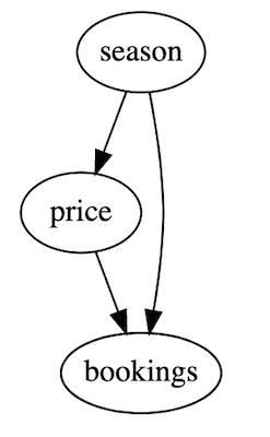
The graph above shows the assumed causal structure of the hotel example. You can clearly see that price causally influences bookings. You can also see that season confounds both price and bookings. Importantly, the DAG also shows which variables we do not take into account. Instead of writing several pages on the different adjustments you did, you now have a single graphic that fits on a powerpoint slide. You can show the DAG to the client and they will immediately see what you did and are able to express concerns if needed. And most importantly, the DAG takes the guesswork away by making your assumptions explicit. No more tables with different adjustments in the appendix. The DAG together with causal inference rules clearly tells you what to adjust for.

You will need to communicate with domain experts in order to make causal inference. Only domain experts can tell you which assumptions are reasonable and well supported by prior research. If your domain experts are no statisticians, they will struggle to formulate their knowledge in statistical terms. Causal graphs make communication with domain experts easy. We could draw them on a whiteboard and the expert could add some nodes and edges or remove them as they see fit. Multiple experts could discuss the DAG. This is not as easy when you are dealing with a set of equations. When quantitative analysts work with C-suite executives, translation of executive knowledge into quantitative terms is often a problem. Causal graphs make this much easier.

How DAGs help identification

The central idea behind modern, graph based causal inference is to use graph theory to identify the variables that need adjustment. In fact, the rules have been made so explicit that a simple algorithm can tell you which variables to adjust for. A key issue these algorithms are looking for is the so called backdoor criterion. Look at the DAG shown above. There is two ways to get from price to bookings: The straight causal arrow which we are investigating, but also a “backdoor path” from price to season to bookings. We can block this backdoor by adjusting for season when estimating the effect of price on bookings.

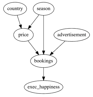
Now let’s look at a bigger graph with some variables added. Which variables do we have to adjust for?

• country only influences price, but not bookings. It does not open a backdoor path and we do not have to adjust for it (but it would not hurt much).

• advertisement equally does not open a backdoor path so we do not have to adjust for it .

• exec_happiness is only influenced by the outcome bookings. Adjusting our statistics for executive happiness would mean we condition on the outcome and introduce selection bias. We must not adjust for it or we would bias our results.

This is why adjusting for all variables we have access too is not a good idea. Either we would adjust unnecessary (usually worsening our statistical results) or we could even introduce bias where there was none before.

This was only a brief guide to the rules behind causal graphs, if you want to learn more I highly recommend Harvard Professor’s Miguel Hernán’s free MOOC on causal graphs.

How computers can help with causal inference

With the rules for identification being encoded in a machine friendly format (find and block the back doors, do not open new back doors), there are several graph based causal inference Python and R packages already. It is still early days in the field, but it can not take long until someone develops an Excel plugin. Causal inference usually does not take much compute power and easily runs on a laptop. It also does not require huge amounts of data. I want to highlight a few useful packages:

• Iain Barr’s CausalGraphicalModels python package makes it easy to work with and understand causal models. I use his software for the examples in this post. He also has an excellent blog series you should check out to learn more.
• For working with data in pandas dataframes Adam Kelleher has a handy python package.
• Laurence Wong’ Causalinference python package provides tools for running the estimation of treatment effects once you have completed the identification. I use this package to estimate the treatment effect in this post.
• Microsoft Research has a python package aiming to automate many steps of the causal inference process
• If you prefer R and work with time series google’s CausalImpact package is for you.

A code example

Back to the hotel example. How can we estimate the true causal effect of price on hotel bookings? We will perform identification using CausalGraphicalModels and then compute the average treatment effect (ATE) using CausalInference. The ATE is the average effect price has on bookings, how much bookings change if we increase the price by one. Since we assume that price has a uniform effect on bookings, we do not have to worry about the effect canceling out in the average.

Identification

For the sake of the example, we will set up a causal model that can also generate samples. Note that we could also perform identification without specifying the treatment effects in advance, but doing so allows us to make sure the our results are correct.

from causalgraphicalmodels.csm import StructuralCausalModel, \
    linear_model
    
hotel = StructuralCausalModel({
    "season": lambda n_samples: np.random.normal(size=n_samples),
    "price": linear_model(["season"],[2]),
    "bookings": linear_model(["season","price"],[5,-1])
})

This causal model will yield the first DAG shown, with seasonality being the only confounder. We can draw the dag with hotel.cgm.draw(). Notice how the true effect of price on bookings specified is -1. Price has a negative effect on bookings, but because season is positively affecting both price and bookings, we see the positive association between price and bookings shown in the first regression plot above.

Just so that we have some data to work with, we will now sample from our model. We could also have used some real world data from a pandas data frame at this point, but sampling directly makes this example easier.

sample = hotel.sample(500)

And now, hold onto your hats, the magic begins: We can query our model for all possible adjustments we could and should do to get a good estimate for the relationship between price and bookings.

hotel.cgm.get_all_backdoor_adjustment_sets("price", "bookings")

The computer can, by itself, figure out what we should adjust for. In this case the result is straightforward: We should adjust for season, and nothing else.

frozenset({frozenset({'season'})})

If this does not stun you, it is worth repeating the exercise with a bigger graph. The fact that a computer can generate the adjustment instructions directly from a graph greatly simplifies causal inference. No more lengthy discussions about what needs to be adjusted for. If we assume that the DAG correctly shows the causal relationships, the computer can directly tell us how to run our inference.

Estimating the treatment effect

Now that we have identified the variable we want to adjust for, estimating the average treatment effect is straightforward using the causalinference package. We only need to specify our outcome, treatment and adjustments:

from causalinference import CausalModel

cm = CausalModel(
    Y=sample["bookings"].values, 
    D=sample["price"].values, 
    X=sample[["season"]].values
)

There are various estimation methods. Since we are dealing only with continuous variables here, we will use linear regression as an estimator. We are interested in the average treatment effect (ATE) as well as the standard error of the treatment effect (for e.g. hypothesis testing). We can obtain both from our estimator:

cm.est_via_ols()

print(f"ATE: {cm.estimates['ols']['ate']:.4f} \
      ATE SE {cm.estimates['ols']['ate_se']:.4f}")

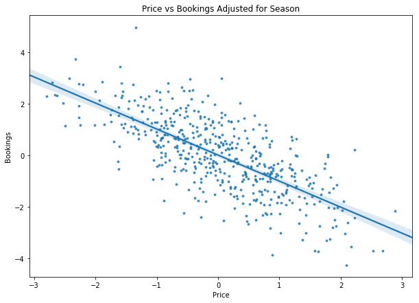
And voila the model clearly shows us that the actual effect of price on bookings is negative.

ATE: -1.0838       ATE SE 0.0558

If we manually adjust the statistics model we can plot the adjusted regression:

It is worth repeating the steps we took to get to this result:

1. We encoded our assumptions about causal relationships into a DAG.
2. The computer used causal inference rules to tell us which variable to adjust for.
3. A stats package automatically computed the average treatment effect with adjusted for the specified variables.

Not only have these steps been relatively straightforward, we can also clearly communicate what we did by putting our DAG on a powerpoint slide and showing it to the client.

But wait there is more

Causal graphs is not the only area in which the field of causal inference has made progress. There are a few notable others:

• Counterfactuals: Would the customer have bought our product if we had lowered the price? Such counterfactual questions can be difficult to answer, since, after all, we did not lower the price and have no data about the customers reaction. However, there has been progress and we can at least make counterfactual predictions, predicting the likelihood of events if something was done differently.

• Examining testable implications: We now have tools to test if our causal assumptions are correct. Our causal graph gives us testable implications and we can examine those to gain confidence in our graph.

• Reasoning about unobserved variables: Sometimes, we can not measure a certain variable. But we can still reason about it, predict it and sometimes even work with an unobserved confounder.

Further reading

I hope that this text has convinced you that causal inference has great value to business analysts and has made great progress. It is now significantly easier to make causal statements with the help of computers. If you would like to dive deeper into causal inference, I recommend the following resources (in increasing order of specialization):

• Judea Pearl’s The Book of Why provides a broad overview into causal inference with a focus on graphical models.
• Miguel Hernán’s free MOOC on causal graphs explains the rules behind causal graphical models in an intuitive way.
• Iain Barr’s blog series on causal inference provides a code heavy introduction with lots of practical tips.
• Hernán and Robins causal inference book is a practical guide using different methods for causal inference.
• Judea Pearl’s Causality is perhaps the standard work for graph based causal inference.

If you enjoyed this post consider subscribing to my newsletter.